Once you start using logistic regression and have come beyond the basic model, you will start going into model diagnostics and comparison of model performances across various peculations for a specific outcome. you will then start coming across concepts of deviance and deviance ratios. Let us understand briefly, how to interpret them.
In order to understand deviance, you need to understand log likelihood.
Log likelihood is a measure of the Goodness of Fit of a model
Likelihood
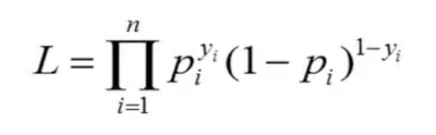
In Logistic regression,
p = predicted probability of event and 1-p is predicted probability of no event.
y =0 if no outcome and y = 1 in case of outcome [ binary 0/1 outcomes in logistic regression]
It follows
py = 1 if y=0
(1-p)1-y = 1 if y = 1
So for an observation the values resolve to:
in case outcome is observed (y is 1) = py = p1 = p
In case outcome is not observed (y is 0) = (1-p)1-0 = 1-p
Likelihood is the multiplication of these values across all observations. [See This YouTube video for detailed explanation].
Log Likelihood
Since Likelihood will become a very small number (we are multiplying so many <1 values after all), It is very difficult to express. We can take its Log and estimate Log Likelihood or LL. Or alternatively we can take Logs of each predicted probability and add them.
Thus in a Logistic regression, the Log-Likelihood is the sum of individual Logs of:
- p: for cases where outcome has happened
- 1–p: for cases where outcome has not happened
across all the observations in a Logistic model.
Since probability is < 1, the Log is negative value, being closer to 0 when probability is high (closer to one) and become more and more negative as the probability reduces towards zero.
We can estimate three types of Log likelihoods
- LLnull = Log likelihood of a Null model that is a model that does not incorporate any variables – This is also sometimes called intercept only model.
- LLsat = Log likelihood of a perfectly fitting or saturated model – likely to be the best possible probability or the LL = 0
- LLproposed = Log likelihood of our fitted proposed model – will lie somewhere in between the null and saturated model
For a Null model, the predicted probability for each sample observation will be set at n/N i.e. the number of outcomes events divided by total sample size and the LLnull will be calculated. This is likely to be the worst or a very negative LL.
For a Saturated model, the predicted probability of each positive outcome is set at one and non-outcome is zero [link]. Since the model perfectly predicts each outcome and non-outcome , the Likelihood ==1 and Log Likelihood = 0
The closer LLproposed is to the saturated model (i.e. LL closer to zero value or Higher Log Likelihood) and away from the null model, better it is.
The differences can be quantified using DEVIANCE.
Deviance
DevianceNull = 2 (LLsat – LLnull) = 2 (0 – LLnull) = -2 LLnull
DevianceResidual = 2 (LLsat – LLproposed) = 2 (0 – LLproposed) = -2LLproposed
Since the LL is a negative value and we are multiplying it by -1, the Deviance becomes a positive value. Therefore a Good model should have as low a DevianceResidual as possible. The Residual Deviance should be lower than null deviance
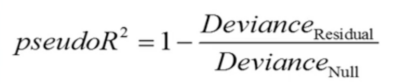
Deviance Ratio
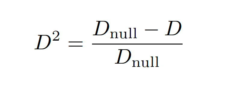
Source: https://www.stata.com/manuals/lassolassogof.pdf See Methods and Formulae
Compare it to the Pseudo R-square formula – They are essentially the same.
Stata Reporting
Stata reports -2LL after every logistic model. So that is the same as deviance.
Stata reports pseudo r square after every logistic model. That is the same as deviance ratio
Stata reports Deviance and Deviance ratios after LASSO logit models in lassogof. These are to be interpreted the same way as LL and pseudo-r-square.
HUGE DISCLAIMER
I am no statistician. I am just trying to understand from various sources and explaining things to myself and hopefully making sense !
Resources