Cheat-sheet
stset failure_time, failure(failure_var == 1) id(id)
stdescribe
* Calculate incidence rates per 1000 , reporting till two decimal places
stptime, per(1000) dd(2)
* Calculate incidence rates per 1000 reporting till two decimal places, at specified time points
stptime, at(7 17 28 90 180 365 ) per(100000) dd(2)
* Calculate incidence rates per 1000 reporting till two decimal places, at specified time points, over sub-groups
stptime, at(7 17 28 90 180 365 ) per(100000) dd(2) by(SurgeryType)
* Kaplan Meier Survival Curve
sts graph
sts graph, by(Gender)
sts graph, by(SurgeryType)
* Nelson Aalen Cumulative Hazard Incidence Curve
sts graph, cumhaz
sts graph, cumhaz by(Gender)
sts graph, cumhaz by(SurgeryType)
* LogRank Test
sts test SurgeryType
********************** Cox Proprotional Hazards Model
stcox i.Gender
stcox i.SurgeryType
stcox i.Gender i.SurgeryType
est drop _all
// risk factors for in SurgeryType ==0
preserve
keep if SurgeryType==0
stcox ib.ageCat i.Gender i.Grp3 i.EC i.SystemicComorb , nolog cformat(%8.2f) pformat(%5.3f)
est store e4 , title("COX_0_HR")
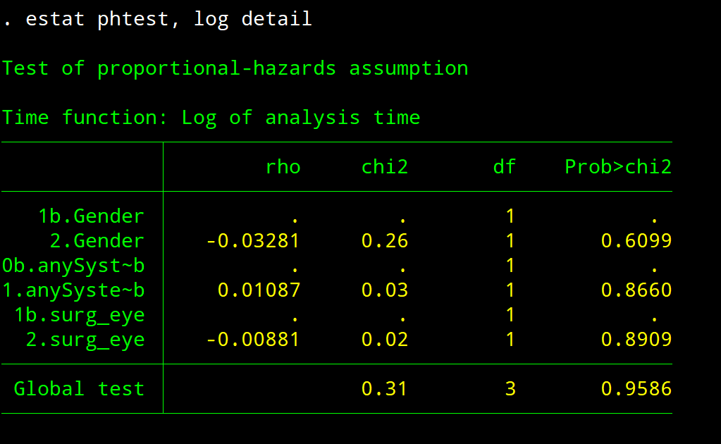
estat phtest, log detail
restore
// and the risk factors in SurgeryType==1
preserve
keep if SurgeryType==1
stcox ib.ageCat i.Gender i.Grp3 i.EC i.SystemicComorb , nolog cformat(%8.2f) pformat(%5.3f)
est store e5 , title("COX_1_HR")
estat phtest, log detail
restore
** COMPARE the outputs of the two models
estout e4 e5 , lab cells("b(fmt(2)) p(fmt(3))") unstack eform stats(r2 bic N)
************************ Test proportionality Assumption
estat phtest, detail // tests the proportional-hazards assumption on the basis of Schoenfeld residuals
// <strong>p-value</strong> of each continuous variable and each category of a categorical variable <strong>must be > 0.05</strong>
* stphtest, log detail
* stphtest is an out-of-date command as of Stata 9
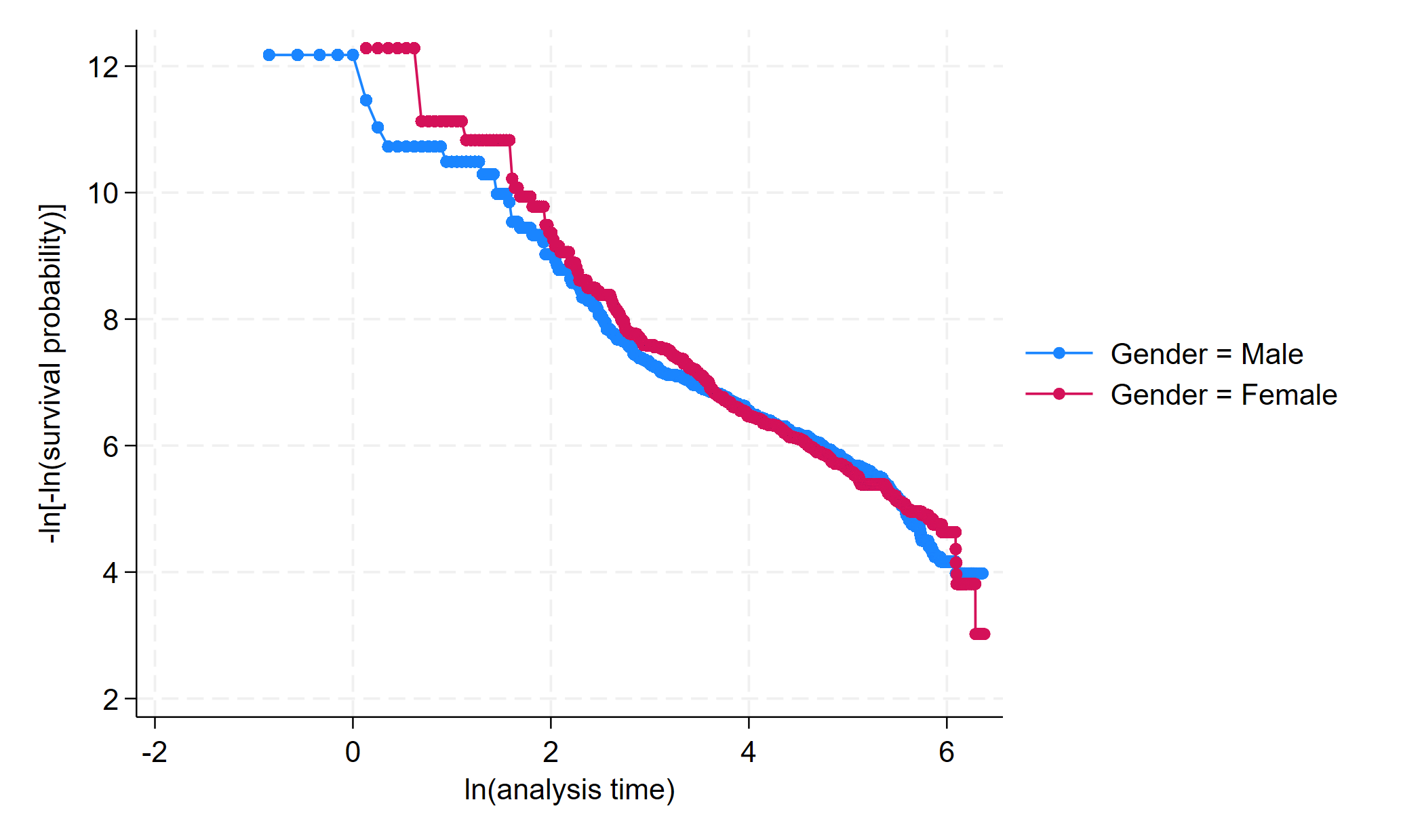
* PH PLot - Lines should be reasonably parallel and must not cross
stphplot, by(SurgeryType)
stphplot, by(SurgeryType) nolntime adjust(i.Gender) ///
plot1opts(symbol(none) color(red) lpattern(dash)) ///
plot2opts(symbol(none) color(navy)) ///
title("Assessment of PH Assumption using log-log plot") ///
subtitle(" Predictor is SurgeryType, adjusted for Gender")
* Compare Kaplan–Meier survival curve with predicted survival from Cox model for each category of Gender
* Observed and predicted Lines should be close to each other
stcoxkm, by(Gender)
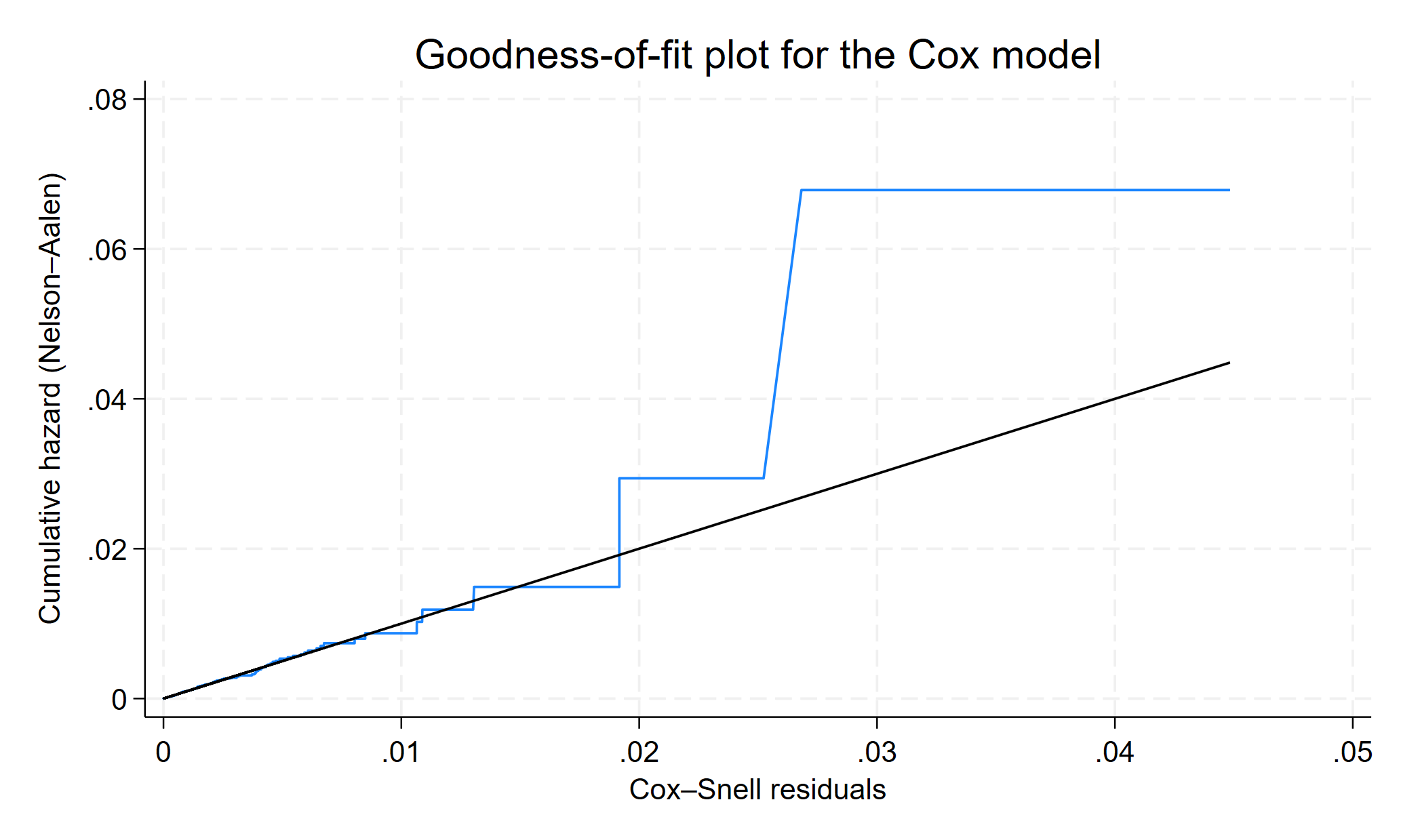
* GOF PLot - plots the estimated cumulative hazard function for the Cox–Snell residuals versus the residuals themselves to assess the goodness of fit of the model visually
Code language: JavaScript (javascript)DETAILS
A Key concept in survival analysis is ANALYSIS TIME. All analyses are performed in terms of time since becoming at risk, called analysis time. Subjects are exposed at t = time = 0 and later fail. Observations with t = time <= 0 are ignored because information before becoming at risk is irrelevant. Subjects May come under observation at any point of time. But that does not define period of risk. Subjects may become at risk at any point of time [origin]. Subjcets who develop a failure event or a censoring event after being at risk are the only ones who considered in Survival analysis.
stset
When id is specified as here, the data are said to be multiple-record data, even if it turns out that there is only one record per subject.
stset failure_time, failure(failure_var == 1) id(id)Here, the failure_var is a categorical variable , coded as 1 for failures. All other values are taken as no failure.
Three more options are important here. origin and enter and exit.
- origin() defines when a subject becomes at risk. All analyses are performed in terms of time since becoming at risk, called analysis time.
- enter() specifies when a subject first comes under observation. In many datasets, becoming at risk and coming under observation are coincident. Then it is sufficient to specify origin().
- exit() specifies the last time under which the subject is both under observation and at risk. exit(failure) is default. However, you can specify additional ouctome categories when subject gets censored
One can specify a time variable for these options . origin(time dob). OR One can specify an categorical variable for these options origin(statusatentry == 2) would mean, for each subject, that the origin time is the earliest time at which statusatentry ==2 is observed. Records before that would be ignored (because t < 0). Subjects who never had statusatentry ==2 would be ignored entirely.
If both timevariable and categories are specified, the latter of the two times is used for origin and enter.
If both timevariable and categories are specified, the earlier of the two times is used for exit
*       Subjects first become at risk at date of birth and
     * come under observation at date of entry into the study
stset dox, id(id) failure(fail) origin(time dob) enter(time doe)

*    Specify the outcome categories 1, 3, and 13 of fail to denote a failure event and
     * the outcome category 5 to indicate that a subject must be removed  from the analysis risk pool
stset dox, id(id) failure(fail==1 3 13) origin(time dob) enter(time doe) exit(fail==1 3 13 5)

* Specify that subjects with dates of exposure dox after 01dec1970 be removed from the analysis risk pool
       * Failure is all non-zero and non-missing values of variable fail
stset dox, failure(fail) origin(time dob) enter(time doe)   exit(time mdy(12,1,1970))Code language: JavaScript (javascript)
scale
You can use scale() with stset to rescale the analysis time. e.g.
- days to weeks:
scale(7)
- days to years
scale(365.25)
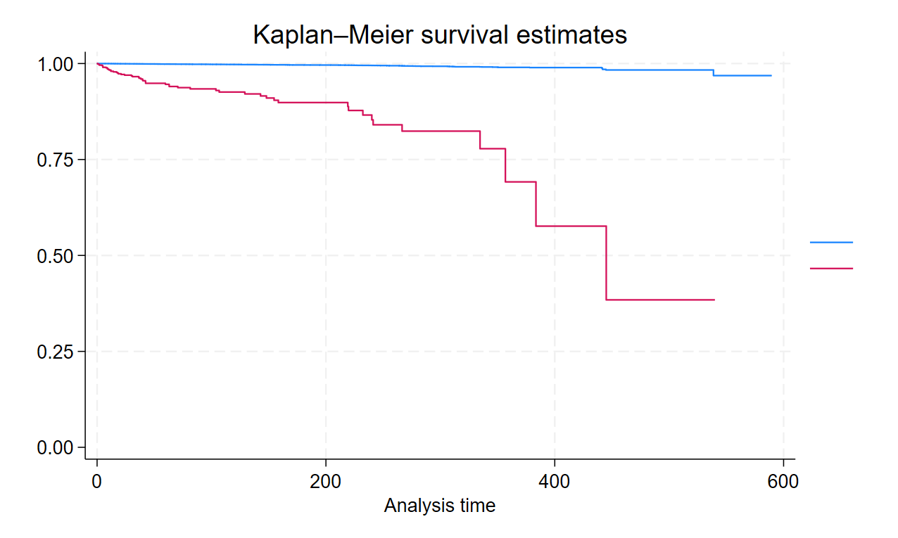
Survival Curve
* Kaplan Meier Survival Curve
sts graph
sts graph, by(Gender)
sts graph, by(SurgeryType)
Cumulative Hazards Curve / Cummulative Incidence Curve / Nelson Aalen Curve
* Nelson Aalen Cumulative Hazard Incidence Curve
sts graph, cumhaz
sts graph, cumhaz by(Gender)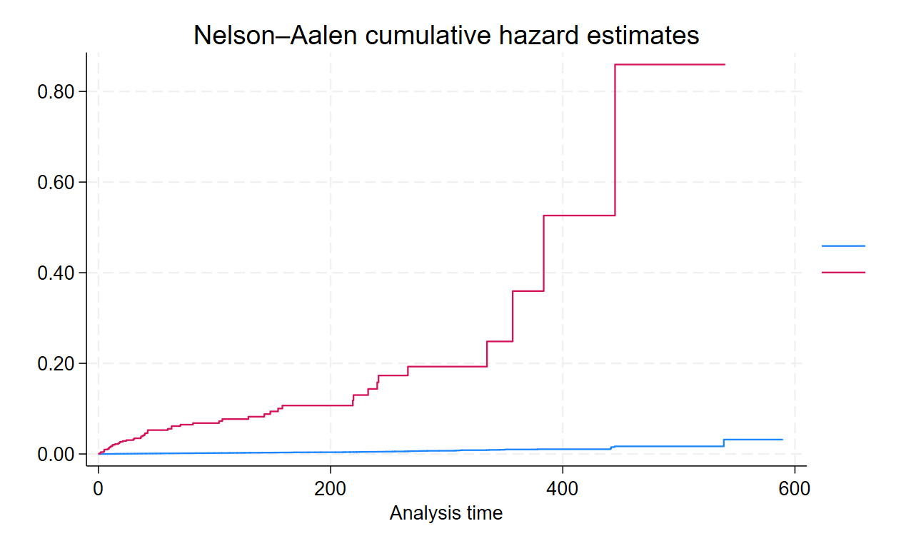
sts test – Log Rank Test
sts test Gender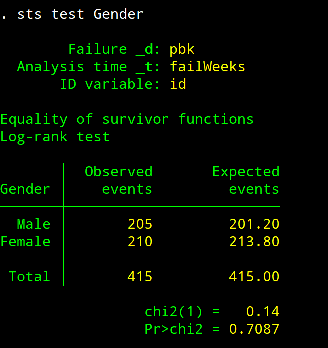
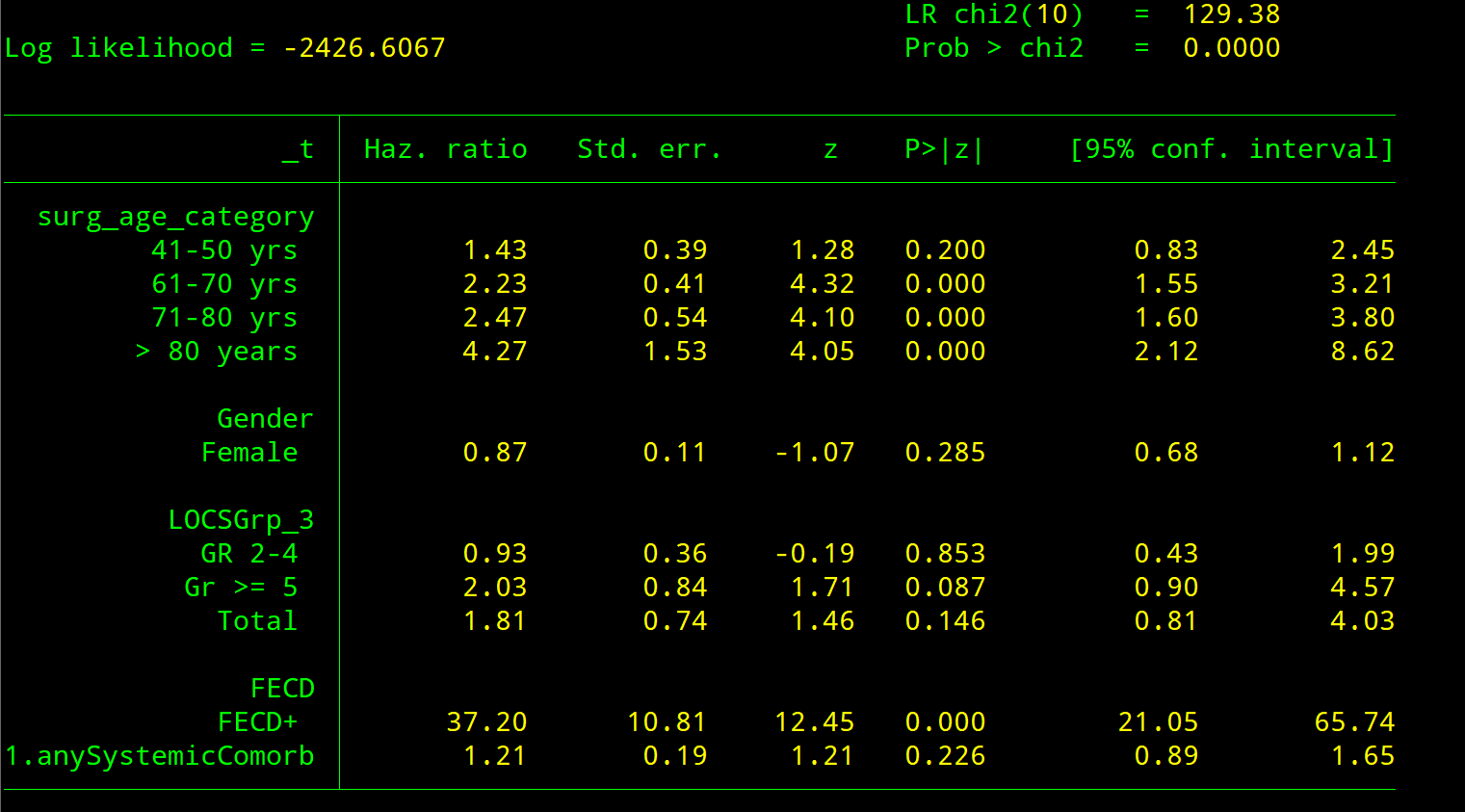
stcox
Use it to run a Cox proprtional Hazards model. This limits the decimals to make results more readable. It also prints the base levels
est drop _all
// risk factors for in  SurgeryType ==0
preserve
keep if SurgeryType==0
stcox ib.ageCat i.Gender  i.Grp3 i.EC i.SystemicComorb , nolog cformat(%8.2f) pformat(%5.3f)
est store e4  , title("COX_0_HR")
estat phtest, log detail
restore


// and the risk factors in SurgeryType==1
preserve
keep if SurgeryType==1
stcox ib.ageCat i.Gender  i.Grp3 i.EC i.SystemicComorb , nolog cformat(%8.2f) pformat(%5.3f)
est store e5  , title("COX_1_HR")
estat phtest, log detail
restore

** COMPARE the outputs of the two models
estout e4 e5 , lab cells("b(fmt(2))  p(fmt(3))") unstack eform stats(r2 bic N)Code language: JavaScript (javascript)
First model
Second model
Get both results in same table
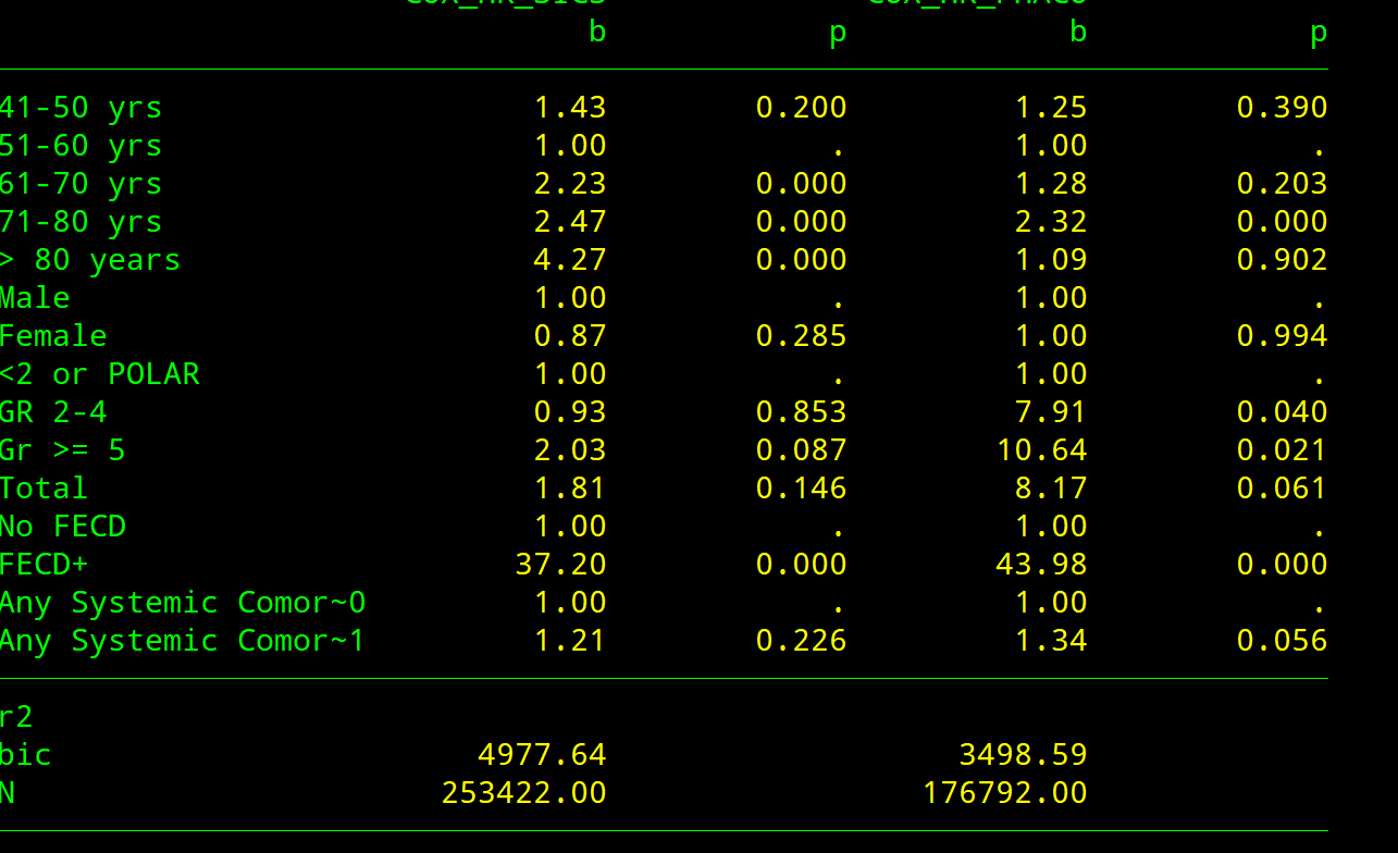
estat phtest, details – Check PH assumption
Both covariate-specific and global tests are reported. rho column reports the correlation between the scaled Schoenfeld residuals and the specified function of time. the p-value of each continuous variable and each category of a categorical variable must be > 0.05. If P of any category of a categorcial variable is < 0.05, then a single HR for that variable is not appropriate.
stphplot
If the plotted lines are reasonably parallel, the proportional-hazards assumption has not been violated, and it would be appropriate to base the estimate for that variable on one baseline survivor function.
GOF PLot
To assess the overall model fit, we can use the Cox–Snell residuals. If the model fits the data, a plot of the cumulative hazard versus the residuals themselves should approximate a straight line with slope 1. This can be done two ways, eirther by using predict after stcox or by using estat gofplot
Compare the jagged line with the reference line for overalao, and see if the Cox model fit these data well or badly
estat gofplot
This command takes away the effort of manually recreating the steps directlty gives us the GOF plot
estat gofplotCheck that the Cox–Snell residuals overlaps teh 45 degree line as much as possible
PREDICT with csnell
The csnell option tells predict to output the Cox–Snell residuals to a new variable. If the Cox regression model fits the data, these residuals should have a standard censored exponential distribution with hazard ratio 1. To check this, we first re-stset the data, specifying cs as our new failure-time variable and same failure/censoring indicator as before
use https://www.stata-press.com/data/r18/drugtr, clear
stset studytime, failure(died)
stcox age drug, nolog

predict cs, csnell
stset cs, failure(died)
sts generate H = na
line H cs cs, sort ytitle("") clstyle(. refline) // We specified cs twice in the graph command above so that a reference 45 degree  line is plottedCode language: JavaScript (javascript)